Spotify-Big-Data-Analysis-Spark
Spotify Big Data Analysis with PySpark
A scalable data engineering and analysis pipeline built on Apache Spark to analyze over 600,000 Spotify tracks spanning a century of recorded music (1921-2020).
Overview
The dataset for this project has 600,000+ records. That is the point where Pandas starts to struggle - slow aggregations, memory warnings, and operations that take minutes instead of seconds. The decision to use Apache Spark was deliberate: this project was built to work the way production data pipelines work, not just to get the analysis done.
Using the PySpark DataFrame API in Google Colab, I built a pipeline that handles ingestion, schema enforcement, dimensionality reduction, temporal aggregation, multi-criteria filtering, and optimized storage - all on a dataset that most classroom tools would choke on.
The Data
| Source | Kaggle - Spotify Dataset 1921-2020 |
| Records | 600,000+ tracks |
| Time Span | 1921-2020 |
| Features | 20 audio and metadata columns |
| Environment | Apache Spark 3.3.0, PySpark, Google Colab |
Pipeline Walkthrough
Schema enforcement on ingestion. The raw CSV was loaded with inferSchema=True and immediately validated with printSchema(). On a dataset this size, letting numeric columns like popularity or energy slip through as strings causes silent failures during aggregations. Catching type mismatches at ingestion is standard practice in production pipelines and I applied it here from the start.
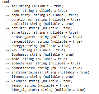
The schema tree confirms correct typing across all 20 columns before any transformations are applied.
Dimensionality reduction. The full dataset has 20 columns. For this analysis, I selected 12 core features - id, name, artists, popularity, year, danceability, energy, loudness, acousticness, instrumentalness, valence, and tempo. Dropping unused columns at this stage reduces memory overhead for every subsequent operation across 600k rows, which compounds meaningfully at this scale.
Temporal trend aggregation (2012-2021). I grouped by year and calculated annual averages for popularity, danceability, and energy to track how the character of popular music shifted over the decade.
yearly_trends = df_selected.groupBy("year").avg("popularity", "danceability", "energy")
yearly_trends.orderBy(col("year").desc()).show(10)
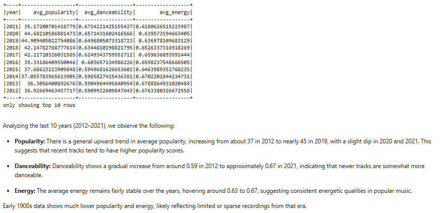
Danceability rose from 0.59 to 0.67 between 2012 and 2021 - a 13.5% increase - while energy levels stayed relatively flat. Modern music has become measurably more danceable without becoming louder or more intense.
Multi-criteria filtering. To simulate a real business request - identifying tracks with high engagement potential - I applied three simultaneous conditions: released after 2000, popularity score of 80 or above, and danceability above 0.7.
filtered_tracks = df_selected.filter(
    (col("year") >= 2000) &
    (col("popularity") >= 80) &
    (col("danceability") > 0.7)
)
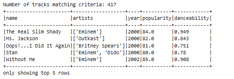
417 tracks met all three criteria. This kind of multi-condition filtering across 600k records runs in under a second with Spark - the same operation in Pandas on a dataset this size would be noticeably slower and more memory-intensive.
Parquet storage for production output. Results were saved in both CSV and Parquet formats. CSV is readable by anyone and easy to share. Parquet is a columnar storage format that provides roughly 3x better compression than CSV and significantly faster read performance for downstream queries in tools like Spark, Hive, or Athena.
yearly_trends.write.mode("overwrite").parquet("yearly_trends.parquet")

Saving to both formats is a common pattern in data engineering - Parquet for the production pipeline, CSV for the stakeholder report.
Key Findings
Danceability in popular music increased 13.5% over the decade from 2012 to 2021, rising from an average of 0.59 to 0.67. Energy levels stayed flat over the same period, which suggests the shift toward more danceable music is driven by rhythm and structure rather than intensity or loudness. Of the 600,000 tracks in the dataset, 417 met the criteria for high popularity (80+) and high danceability (0.7+) released after 2000.
Repository Structure
Spotify-Big-Data-Analysis-Spark/
│
├── Spotify Data Analysis Spark.ipynb   # Full pipeline - ingestion, cleaning, analysis, storage
├── schema_tree.png                     # Schema validation output
├── yearly_trends.png                   # Temporal aggregation results
├── viral_tracks.png                    # Filtered high-engagement tracks
├── persistence_code.png                # CSV and Parquet write operations
└── README.md
Limitations and What I Would Do Differently
The analysis is limited to audio features already present in the dataset - there is no streaming data, no play count, and no listener demographic information. Popularity scores are a Spotify-calculated metric whose exact formula is not public, which means the filtering threshold of 80 is directionally useful but not precisely defined.
If I were extending this project, I would connect to the Spotify API directly to pull live streaming data, add a machine learning layer to predict track popularity from audio features, and run the pipeline on a proper distributed cluster rather than a single Colab instance to demonstrate true horizontal scaling.
Tools
Apache Spark 3.3.0, PySpark, Python, Google Colab
About Me
Tejashwini Saravanan - Master’s student in Data Analytics with a focus on scalable data pipelines and making complex data legible and actionable.